API
Table
|
Convert the coefficients to real space |
|
Calculate 2-point stats for a multiple auto/cross correlation |
|
Generate a 2-phase checkerboard microstructure |
|
Generate a delta microstructure |
|
Constructs microstructures for an arbitrary number of phases given the size of the domain, and relative grain size. |
|
Compute graph descriptors for multiple samples |
|
Computes the pair correlations from 2-point statistics. |
|
Plot a set of microstructures side-by-side |
|
Solve the Cahn-Hilliard equation. |
|
Solve the elasticity problem |
|
Run all the module tests. |
|
Calculate the 2-points stats for two arrays |
Reshape data ready for a PCA. |
|
|
Make a generic transformer based on a function |
|
Calculate GraphDescriptors as part of a Sklearn pipeline |
|
Legendre transformer for Sklearn pipelines |
|
Perform the localization in Sklearn pipelines |
|
Primitive transformer for Sklearn pipelines |
|
Reshape data ready for the LocalizationRegressor |
|
Calculate the 2-point stats for two arrays as part of Scikit-learn pipeline. |
Functions
- pymks.coeff_to_real(coeff='__no__default__', new_shape=None)
Convert the coefficients to real space
Convert the
pymks.LocalizationRegressorcoefficiencts to real space. The coefficiencts are calculated in Fourier space, but best viewed in real space. If the Fourier coefficients are defined as \(\beta\left[l, k\right]\) then the real space coefficients are calculated using,\[\alpha \left[l, r\right] = \frac{1}{N} \sum_{k=0}^{N-1} \beta\left[l, k\right] e^{i \frac{2 \pi}{N} k r} e^{i \pi}\]where \(l\) is the local state and \(r\) is the spatial index from \(0\) to \(N-1\). The \(e^{i \pi}\) term is a shift applied to place the 0 coefficient at the center of the domain for viewing purposes.
- Parameters
coeff (array) – the localization coefficients in Fourier space as a Dask array (n_x, n_y, n_state)
new_shape (tuple) – shape of the output to either shorten or pad with zeros
- Returns
the coefficients in real space
A spike at \(k=1\) should result in a cosine function on the real axis.
>>> N = 100
>>> fcoeff = np.zeros((N, 1))
>>> fcoeff[1] = N
>>> x = np.linspace(0, 1, N + 1)[:-1]
>>> assert np.allclose(
...     coeff_to_real(da.from_array(fcoeff)).real.compute(),
...     np.cos(2 * np.pi * x + np.pi)[:, None]
... )
- pymks.correlations_multiple(data, correlations, periodic_boundary=True, cutoff=None)
Calculate 2-point stats for a multiple auto/cross correlation
The discretized two point statistics are given by
\[f[r \; \vert \; l, l'] = \frac{1}{S} \sum_s m[s, l] m[s + r, l']\]where \(f[r \; \vert \; l, l']\) is the conditional probability of finding the local states \(l\) and \(l'\) at a distance and orientation away from each other defined by the vector \(r\). See this paper for more details on the notation.
The correlations are calulated based on pairs given in
correlationsfor each sample.To calculate a single correlation for two arrays, see
two_point_stats().To use
correlations_multipleas part of a Scikit-learn pipeline, seeTwoPointCorrelation.- Parameters
data – the discretized data with shape
(n_samples, n_x, n_y, n_state)correlations – the correlation pairs,
[[i0, j0], [i1, j1], ...]periodic_boundary – whether to assume a periodic boundary (default is true)
cutoff – the subarray of the 2 point stats to keep
- Returns
the 2-points stats array
If
datais a Numpy array thencorrelations_multiplewill return a Numpy array.>>> data = np.arange(18).reshape(1, 3, 3, 2) >>> out_np = correlations_multiple(data, [[0, 1], [1, 1]]) >>> out_np.shape (1, 3, 3, 2) >>> answer = np.array([[[58, 62, 58], [94, 98, 94], [58, 62, 58]]]) + 2. / 3. >>> assert np.allclose(out_np[..., 0], answer)
However, if
datais a Dask array then a Dask array is returned.>>> data = da.from_array(data, chunks=(1, 3, 3, 2)) >>> out = correlations_multiple(data, [[0, 1], [1, 1]]) >>> out.shape (1, 3, 3, 2) >>> out.chunks ((1,), (3,), (3,), (2,)) >>> assert np.allclose(out[..., 0], answer)
- pymks.generate_checkerboard(size, square_shape=(1,))
Generate a 2-phase checkerboard microstructure
- Parameters
size (tuple) – the size of the domain
(n_x, n_y)square_shape (tuple) – the shape of each subdomain
(n_x, n_y)
- Returns
a microstructure of shape (1,) + shape (extra sample axis)
>>> print(generate_checkerboard((4,)).compute())
[[0 1 0 1]]
>>> print(generate_checkerboard((3, 3)).compute())
[[[0 1 0]
  [1 0 1]
  [0 1 0]]]
>>> print(generate_checkerboard((3, 3), (2,)).compute())
[[[0 0 1]
  [0 0 1]
  [1 1 0]]]
>>> print(generate_checkerboard((5, 8), (2, 3)).compute())
[[[0 0 0 1 1 1 0 0]
  [0 0 0 1 1 1 0 0]
  [1 1 1 0 0 0 1 1]
  [1 1 1 0 0 0 1 1]
  [0 0 0 1 1 1 0 0]]]
- pymks.generate_delta(n_phases='__no__default__', shape='__no__default__', chunks=())
Generate a delta microstructure
A delta microstructure has a 1 at the center and 0 everywhere else for each phase. This is used to calibrate linear elasticity models that only require delta microstructures for calibration.
- Parameters
n_phases (int) – number of phases
shape (tuple) – the shape of the microstructure,
(n_x, n_y)chunks (tuple) – how to chunk the sample axis
(n_chunk,)
- Returns
a dask array of delta microstructures
If n_phases=5 for example, this requires 20 microstructures as each phase pairing requies 2 microstructure arrays.
>>> arr = generate_delta(5, (3, 4), chunks=(5,))
>>> arr.shape
(20, 3, 4)
>>> arr.chunks
((5, 5, 5, 5), (3,), (4,))
>>> print(arr[0].compute())
[[0 0 0 0]
 [0 0 1 0]
 [0 0 0 0]]
generate_delta requires at least 2 phases
>>> arr = generate_delta(2, (3, 3))
>>> arr.shape
(2, 3, 3)
>>> print(arr[0].compute())
[[0 0 0]
 [0 1 0]
 [0 0 0]]
- pymks.generate_multiphase(shape='__no__default__', grain_size='__no__default__', volume_fraction='__no__default__', chunks=- 1, percent_variance=0.0, seed=None)
Constructs microstructures for an arbitrary number of phases given the size of the domain, and relative grain size.
- Parameters
shape (tuple) – shape of the domain
(n_sample, n_x, n_y)grain_size (tuple) – typical expected grain size
(n_x, n_y)volume_fraction (tuple) – the percent volume fraction for each phase, which must sum to 1
chunks (int) – chunks_size of the sample index
percent_variance (float) – the percent variance for each value of volume_fraction
seed (int) – set the seed value, default is no seed
- Returns
A dask array of random-multiphase microstructures microstructures for the system of shape given by shape.
Example:
>>> x_expected = np.array([[[0, 0, 0],
...                         [0, 1, 0],
...                         [1, 1, 1]]])
>>> x_actual = generate_multiphase(
...     shape=(1, 3, 3),
...     grain_size=(1, 1),
...     volume_fraction=(0.5, 0.5),
...     seed=10
... )
>>> print(x_actual.shape)
(1, 3, 3)
>>> assert np.allclose(x_actual, x_expected)
If chunks is not set a Numpy array is returned.
>>> type(x_actual)
<class 'numpy.ndarray'>
If chunks is defined a Dask array is returned.
>>> x = generate_multiphase(
...     shape=(2, 3, 3),
...     grain_size=(1, 1),
...     volume_fraction=(0.5, 0.5),
...     chunks=1
... )
>>> print(x.chunks)
((1, 1), (3,), (3,))
- pymks.graph_descriptors(data='__no__default__', delta_x=1.0, periodic_boundary=True)
Compute graph descriptors for multiple samples
- Parameters
data – array of phases (n_samples, n_x, n_y), values must be 0 or 1
delta_x – pixel size
periodic_boundary – whether the boundaries are periodic
- Returns
A Pandas data frame with samples along rows and descriptors along columns
Compute graph descriptors for multiple samples using the GraSPI sub-package. See the installation instructions to install PyMKS with GraSPI enabled.
GraSPI is focused on characterizing photovoltaic devices and so the descriptors must be understood in this context. Future releases will have more generic descriptors. See Wodo et al. for more details. Note that the current implementation only works for two phase data.
This function returns a Pandas Dataframe with the descriptors as columns and samples in rows. In the context of a photovoltaic device the top of the domain (y-direction) represents an anode and the bottom of the domain represents a cathode. Phase 0 represents donor materials while phase 1 represents acceptor material. Many of these descriptors characterizes the morphology in terms of hole electron pair generation and transport leading to device charge extraction.
To use graph_descriptors as part of a Sklearn pipeline, see
GraphDescriptors.The column descriptors are as follows.
Column Name
Description
n_vertices
The number of vertices in the constructed graph. Should be equal to the number of pixels.
n_edges
The number of edges in the constructed graph.
n_phase{i}
The number of vertices for phase {i}.
n_phase{i}_connect
The number of connected components for phase {i}.
n_phase{i}_connect_top
The number of connected components for phase {i} with the top of the domain in y-direction.
n_phase{i}_connect_bottom
The number of connected components for phase {i} with the top of the domain in y-direction.
w_frac_phase{i}
Weighted fraction of phase {i} vertices.
frac_phase{i}
Fraction of phase {i} vertices.
w_frac_phase{i}_{j}_dist
Weighted fraction of phase {i} vertices within j nodes from an interface.
frac_phase{i}_{j}_dist
Fraction of phase {i} vertices within {j} nodes from an interface.
frac_useful
Fraction of useful vertices connected the top or bottom of the domain.
inter_frac_bottom_top
Fraction of interface with complementary paths to bottom or top of the domain.
frac_phase{i}_top
Fraction of phase {i} interface vertices with path to top.
frac_phase{i}_bottom
Fraction of phase {i} interface vertices with path to bottom.
n_inter_paths
Number of interface edges with complementary paths.
n_phase{i}_inter_top
Number of phase {i} interface vertices with path to top
n_phase{i}_inter_bottom
Number of phase {i} interface vertices with path to bottom
frac_phase{i}_rising
Fraction of phase {i} with rising paths
Example, with 3 x (3, 3) arrays
Read in the expected data.
>>> from io import StringIO
>>> expected = pandas.read_csv(StringIO('''
... n_vertices,n_edges,n_phase0,n_phase1,n_phase0_connect,n_phase1_connect,n_phase0_connect_top,n_phase1_connect_bottom,w_frac_phase0,frac_phase0,w_frac_phase0_10_dist,fraction_phase0_10_dist,inter_frac_bottom_and_top,frac_phase0_top,frac_phase1_bottom,n_inter_paths,n_phase0_inter_top,n_phase1_inter_bottom,frac_phase0_rising,frac_phase1_rising,n_phase0_connect_anode,n_phase1_connect_cathode
... 9,7,3,6,2,1,1,1,0.3256601095199585,0.3333333432674408,0.9624541997909546,1.0,0.4285714328289032,0.3333333432674408,1.0,3,1,6,1.0,0.6666666865348816,2,2
... 9,6,3,6,1,1,1,1,0.3267437815666199,0.3333333432674408,0.9624541997909546,1.0,1.0,1.0,1.0,6,3,6,1.0,1.0,2,3
... 9,6,6,3,2,1,1,0,0.6534984707832336,0.6666666865348816,0.9624541997909546,1.0,0.0,0.5,0.0,0,3,0,1.0,0.0,4,1
... '''))
Construct the 3 samples each with 3x3 voxels
>>> data = np.array([[[0, 1, 0],
...                   [0, 1, 1],
...                   [1, 1, 1]],
...                  [[1, 1, 1],
...                   [0, 0, 0],
...                   [1, 1, 1]],
...                  [[0, 1, 0],
...                   [0, 1, 0],
...                   [0, 1, 0]]])
>>> actual = graph_descriptors(data)
graph_descriptorsreturns a data frame.>>> actual n_vertices n_edges ... n_phase0_connect_anode n_phase1_connect_cathode 0 9 7 ... 2 2 1 9 6 ... 2 3 2 9 6 ... 4 1 [3 rows x 22 columns]
Check that the actual values are equal to the expected values.
>>> assert np.allclose(actual, expected)
Works with Dask arrays as well. When using Dask a Dask dataframe will be returned.
>>> import dask.array as da
>>> out = graph_descriptors(da.from_array(data, chunks=(2, 3, 3)))
>>> out.get_partition(0).compute()
   n_vertices  n_edges  ...  n_phase0_connect_anode  n_phase1_connect_cathode
0           9        7  ...                       2                         2
1           9        6  ...                       2                         3

[2 rows x 22 columns]
On examining the data for this simple test case there are a few obvious checks. Each sample has 9 vertices since there are 9 pixels in each sample.
>>> actual.n_vertices
0    9
1    9
2    9
Name: n_vertices, dtype: int64
Notice that the first and third sample have two phase 1 regions connected to either the top or bottom of the domain while the second sample has only 1 region.
>>> actual.n_phase1_connect
0    1
1    1
2    1
Name: n_phase1_connect, dtype: int64
All paths are blocked for the first and second samples from reaching the top from the bottom surface. The third sample has 6 interface edges that connect the top and bottom.
>>> actual.n_inter_paths
0    3
1    6
2    0
Name: n_inter_paths, dtype: int64
- pymks.paircorr_from_twopoint(x_data, cutoff_r=None, interpolate_n=None)
Computes the pair correlations from 2-point statistics.
The pair correlations are the radial average of the 2 point stats. The grid spacing is assumed to be one unit. Linear interpolation is used if
interpolate_nis specified. If another interpolation is desired, don’t specify this parameter and perform desired interpolation on the output.The discretized two point statistics are given by
\[f[r \; \vert \; l, l'] = \frac{1}{S} \sum_s m[s, l] m[s + r, l']\]where \(f[r \; \vert \; l, l']\) is the conditional probability of finding the local states \(l\) and math:l’ at a distance and orientation away from each other defined by the vector \(r\). See this paper for more details on the notation.
The pair correlation is defined as the conditional probability for the case of the magnitude vector, \(||r||_2\), defined by \(g[d]\). \(g\) is related to \(f\) via the following transformation. Consider the set, \(I[d] := \{ f[r] \; \vert \; ||r||_2 = d \}\) then
\[g[d] = \frac{1}{ | I[ d ] | } \sum_{f \in I[ d ]} f\]The \(d\) are radii from the center pixel of the domain. They are automatially calculated if
interpolate_nisNone.It’s assumed that
x_datais a valid set of two point statistics calculated from the PyMKS correlations module.- Parameters
x_data – array of centered 2-point statistics. (n_samples, n_x, n_y, …)
cutoff_r – the radius cut off. Values less than 1 are assumed to be a proportion while values greater than 1 are an exact radius cutoff
interpolate_n – the number of equally spaced radii that the probabilities will be interpolated to
- Returns
A tuple of the pair correlation array and the radii cutoffs used for averaging or interpolation. The pair correlations are shaped as
(n_samples, n_radii), whilst the radii are shaped as(n_radii,).n_radiiis equal tointerpolate_nwheninterpolate_nis specified. The probabilities are chunked on the sample axis the same asx_data. The radii is a numpy array.
Test with only 2 samples of 3x3
>>> import dask.array as da
>>> x_data = np.array([
...     [
...         [0.2, 0.4, 0.3],
...         [0.4, 0.5, 0.5],
...         [0.2, 0.5, 0.3]
...     ],
...     [
...         [0.1, 0.2, 0.3],
...         [0.2, 0.6, 0.4],
...         [0.1, 0.4, 0.3]
...     ]
... ])
Most basic test
>>> probs, radii = paircorr_from_twopoint(x_data)
>>> assert np.allclose(probs,
...     [[0.5, 0.45, 0.25],
...      [0.6, 0.3, 0.2]])
>>> assert np.allclose(radii, [0, 1, np.sqrt(2)])
Test with
cutoff_rgreater than 1>>> probs, radii = paircorr_from_twopoint(x_data, cutoff_r=1.01) >>> assert np.allclose(probs, ... [[0.5, 0.45], ... [0.6, 0.3]]) >>> assert np.allclose(radii, [0, 1])
Test with
cutoff_rless than 1>>> probs, radii = paircorr_from_twopoint(x_data, cutoff_r=0.99) >>> assert np.allclose(probs, ... [[0.5, 0.45], ... [0.6, 0.3]]) >>> assert np.allclose(radii, [0, 1])
Test with a linear interpolation
>>> probs, radii = paircorr_from_twopoint(x_data, interpolate_n=2)
>>> assert np.allclose(probs,
...     [[0.5, 0.25],
...      [0.6, 0.2]])
>>> assert np.allclose(radii, [0, np.sqrt(2)])
Test with Dask. The chunks along the sample axis are preserved.
>>> arr = da.from_array(np.random.random((10, 4, 3, 3)), chunks=(2, 4, 3, 3))
>>> probs, radii = paircorr_from_twopoint(arr)
>>> probs.shape
(10, 7)
>>> probs.chunks
((2, 2, 2, 2, 2), (7,))
>>> assert np.allclose(radii, np.sqrt([0, 1, 2, 3, 4, 5, 6]))
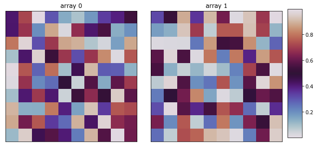
- pymks.plot_microstructures(*arrs, titles=(), cmap=None, colorbar=True, showticks=False, figsize_weight=4)
Plot a set of microstructures side-by-side
- Parameters
arrs – any number of 2D arrays to plot
titles – a sequence of titles with len(*arrs)
cmap – any matplotlib colormap
>>> import numpy as np
>>> np.random.seed(1)
>>> x_data = np.random.random((2, 10, 10))
>>> fig = plot_microstructures(
...     x_data[0],
...     x_data[1],
...     titles=['array 0', 'array 1'],
...     cmap='twilight'
... )
>>> fig.show()
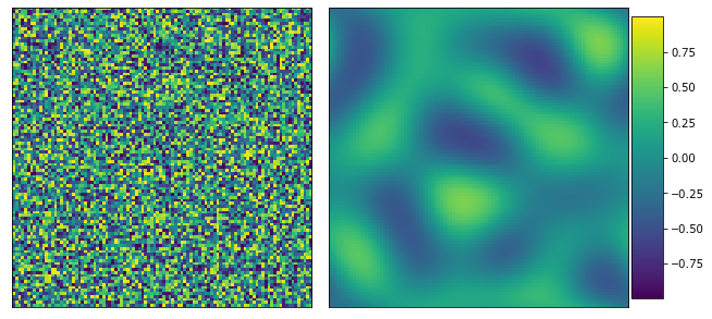
- pymks.solve_cahn_hilliard(x_data, n_steps=1, delta_x=0.25, delta_t=0.001, gamma=1.0)
Solve the Cahn-Hilliard equation.
Solve the Cahn-Hilliard equation for multiple samples in arbitrary dimensions. The concentration varies from -1 to 1. The equation is given by
\[\dot{\phi} = \nabla^2 \left( \phi^3 - \phi \right) - \gamma \nabla^4 \phi\]The discretiztion scheme used here is from Chang and Rutenberg. The scheme is a semi-implicit discretization in time and is given by
\[\phi_{t+\Delta t} + \left(1 - a_1\right) \Delta t \nabla^2 \phi_{t+\Delta t} + \left(1 - a_2\right) \Delta t \gamma \nabla^4 \phi_{t+\Delta t} = \phi_t - \Delta t \nabla^2 \left(a_1 \phi_t + a_2 \gamma \nabla^2 \phi_t - \phi_t^3 \right)\]where \(a_1=3\) and \(a_2=0\).
- Parameters
x_data – dask array chunked along the sample axis
(n_sample, n_x, n_y)n_steps – number of time steps used
delta_x – the grid spacing, \(\Delta x\)
delta_t – the time step size, \(\Delta t\)
gamma – Cahn-Hilliard parameter, \(\gamma\)
>>> import dask.array as da
>>> da.random.seed(99)
>>> x_data = 2 * da.random.random((1, 100, 100), chunks=(1, 100, 100)) - 1
>>> y_data = solve_cahn_hilliard(x_data)
>>> y_data.chunks
((1,), (100,), (100,))
>>> y_data = solve_cahn_hilliard(x_data, n_steps=10000)
>>> from pymks import plot_microstructures
>>> fig = plot_microstructures(x_data[0], y_data[0])
>>> fig.show()
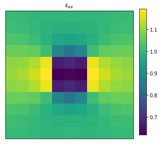
- pymks.solve_fe(x_data='__no__default__', elastic_modulus='__no__default__', poissons_ratio='__no__default__', macro_strain=1.0, delta_x=1.0)
Solve the elasticity problem
Use Sfepy to solve a linear strain problem in 2D with a varying microstructure on a rectangular grid. The rectangle (cube) is held at the negative edge (plane) and displaced by 1 on the positive x edge (plane). Periodic boundary conditions are applied to the other boundaries.
The boundary conditions on the rectangle (or cube) are given by
\[u(L, y) = L \left(1 + \bar{\varepsilon}_{xx}\right)\]\[u(0, L) = u(0, 0) = 0\]\[u(x, 0) = u(x, L)\]where \(\bar{\varepsilon}_{xx}\) is the
macro_strain, \(u\) is the displacement in the \(x\) direction, and \(L\) is the length of the domain. More details about these boundary conditions can be found in Landi et al.See the elasticity notebook for a full set of equations.
x_datashould have integer values that represent the phase of the material. The integer values should correspond to the indices for theelastic_modulusandpoisson_ratiosequences and, therefore,elastic_modulusandpoisson_rationeed to be of the same length.- Parameters
x_data – microstructures with shape,
(n_samples, n_x, ...)elastic_modulus – the elastic modulus in each phase,
(e0, e1, ...)poissons_ratio – the poissons ratio for each phase,
(p0, p1, ...)macro_strain – the macro strain, \(\bar{\varepsilon}_{xx}\)
delta_x – the grid spacing
- Returns
a dictionary of strain, displacement and stress with stress and strain of shape
(n_samples, n_x, ..., 3)and displacement shape of(n_samples, n_x + 1, ..., 2)
>>> import numpy as np
>>> x_data = np.zeros((1, 11, 11), dtype=int)
>>> x_data[0, :, 1] = 0
x_datahas values of 0 and 1 and soelastic_modulusandpoisson_ratiomust each have 2 entries for phase 0 and phase 1.>>> strain = solve_fe( ... x_data, ... elastic_modulus=(1.0, 10.0), ... poissons_ratio=(0., 0.), ... macro_strain=1., ... delta_x=1. ... )['strain']
>>> from pymks import plot_microstructures
>>> fig = plot_microstructures(strain[0, ..., 0], titles=r'$\varepsilon_{xx}$')
>>> fig.show()
- pymks.test(*args)
Run all the module tests.
Equivalent to running
py.test pymksin the base of PyMKS. Allows an installed version of PyMKS to be tested.- Parameters
*args – add arguments to pytest
To test an installed version of PyMKS use
$ python -c "import pymks; pymks.test()"
- pymks.two_point_stats(arr1='__no__default__', arr2='__no__default__', periodic_boundary=True, cutoff=None, mask=None)
Calculate the 2-points stats for two arrays
The discretized two point statistics are given by
\[f[r \; \vert \; l, l'] = \frac{1}{S} \sum_s m[s, l] m[s + r, l']\]where \(f[r \; \vert \; l, l']\) is the conditional probability of finding the local states \(l\) and \(l\) at a distance and orientation away from each other defined by the vector \(r\). See this paper for more details on the notation.
The array
arr1[i](state \(l\)) is correlated witharr2[i](state \(l'\)) for each samplei. Both arrays must have the same number of samples and nominal states (integer value) or continuous variables.To calculate multiple different correlations for each sample, see
correlations_multiple().To use
two_point_statsas part of a Scikit-learn pipeline, seeTwoPointCorrelation.- Parameters
arr1 – array used to calculate cross-correlations, shape
(n_samples,n_x,n_y)arr2 – array used to calculate cross-correlations, shape
(n_samples,n_x,n_y)periodic_boundary – whether to assume a periodic boundary (default is
True)cutoff – the subarray of the 2 point stats to keep
mask – array specifying confidence in the measurement at a pixel, shape
(n_samples,n_x,n_y). In range [0,1].
- Returns
the snipped 2-points stats
If both arrays are Dask arrays then a Dask array is returned.
>>> out = two_point_stats(
...     da.from_array(np.arange(10).reshape(2, 5), chunks=(2, 5)),
...     da.from_array(np.arange(10).reshape(2, 5), chunks=(2, 5)),
... )
>>> out.chunks
((2,), (5,))
>>> out.shape
(2, 5)
If either of the arrays are Numpy then a Numpy array is returned.
>>> two_point_stats(
...     np.arange(10).reshape(2, 5),
...     np.arange(10).reshape(2, 5),
... )
array([[ 3.,  4.,  6.,  4.,  3.],
       [48., 49., 51., 49., 48.]])
Test masking
>>> array = da.array([[[1, 0 ,0], [0, 1, 1], [1, 1, 0]]])
>>> mask = da.array([[[1, 1, 1], [1, 1, 1], [1, 0, 0]]])
>>> norm_mask = da.array([[[2, 4, 3], [4, 7, 4], [3, 4, 2]]])
>>> expected = da.array([[[1, 0, 1], [1, 4, 1], [1, 0, 1]]]) / norm_mask
>>> assert np.allclose(
...     two_point_stats(array, array, mask=mask, periodic_boundary=False)[:, 1:-1, 1:-1],
...     expected
... )
The mask must be in the range 0 to 1.
>>> array = da.array([[[1, 0], [0, 1]]])
>>> mask =  da.array([[[2, 0], [0, 1]]])
>>> two_point_stats(array, array, mask=mask)
Traceback (most recent call last):
...
RuntimeError: Mask must be in range [0,1]
Classes
- class pymks.FlattenTransformer
Reshape data ready for a PCA.
Two point correlation data need to be flatten before performing PCA. This class flattens the two point correlation data for use in a Sklearn pipeline.
>>> data = np.arange(50).reshape((2, 5, 5))
>>> FlattenTransformer().transform(data).shape
(2, 25)
- fit(*_)
Only necessary to make pipelines work
- static transform(x_data)
Transform the X data
- Parameters
x_data – the data to be transformed
- class pymks.GenericTransformer(func)
Make a generic transformer based on a function
>>> import numpy as np
>>> data = np.arange(4).reshape(2, 2)
>>> GenericTransformer(lambda x: x[:, 1:]).fit(data).transform(data).shape
(2, 1)
Instantiate a GenericTransformer
Function should take a multi-dimensional array and return an array with the same length in the sample axis (first axis).
- Parameters
func – transformer function
- fit(*_)
Only necessary to make pipelines work
- transform(data)
Transform the data
- Parameters
data – the data to be transformed
- Returns
the transformed data
- class pymks.GraphDescriptors(delta_x=1.0, periodic_boundary=True)
Calculate GraphDescriptors as part of a Sklearn pipeline
Wraps the
graph_descriptors()functionTest
>>> data = np.array([[[0, 1, 0],
...                   [0, 1, 1],
...                   [1, 1, 1]],
...                  [[1, 1, 1],
...                   [0, 0, 0],
...                   [1, 1, 1]],
...                  [[0, 1, 0],
...                   [0, 1, 0],
...                   [0, 1, 0]]])
>>> actual = GraphDescriptors().fit(data).transform(data)
>>> actual.shape
(3, 22)
See the
graph_descriptors()function for more complete documentation.Instantiate a GraphDescriptors transformer
- Parameters
delta_x – pixel size
periodic_boundary – whether the boundaries are periodic
columns – subset of columns to include
- fit(*_)
Only necessary to make pipelines work
- transform(data)
Transform the data
- Parameters
data – the data to be transformed
- Returns
the graph descriptors dataframe
- class pymks.LegendreTransformer(n_state=2, min_=0.0, max_=1.0, chunks=None)
Legendre transformer for Sklearn pipelines
>>> from toolz import pipe
>>> data = da.from_array(np.array([[0, 0.5, 1]]), chunks=(1, 3))
>>> pipe(
...     LegendreTransformer(),
...     lambda x: x.fit(None, None),
...     lambda x: x.transform(data).compute(),
... )
array([[[ 0.5, -1.5],
        [ 0.5,  0. ],
        [ 0.5,  1.5]]])
Instantiate a LegendreTransformer
- Parameters
n_state – the number of local states
min – the minimum local state
max – the maximum local state
chunks – chunks size for state axis
- class pymks.LocalizationRegressor(redundancy_func=<function LocalizationRegressor.<lambda>>)
Perform the localization in Sklearn pipelines
Allows the localization to be part of a Sklearn pipeline
>>> make_data = lambda s, c: da.from_array(
...     np.arange(np.prod(s),
...               dtype=float).reshape(s),
...     chunks=c
... )
>>> X = make_data((6, 4, 4, 3), (2, 4, 4, 1))
>>> y = make_data((6, 4, 4), (2, 4, 4))
>>> y_out = LocalizationRegressor().fit(X, y).predict(X)
>>> assert np.allclose(y, y_out)
>>> print(
...     pipe(
...         LocalizationRegressor(),
...         lambda x: x.fit(X, y.reshape(6, 16)).predict(X).shape
...     )
... )
(6, 16)
Instantiate a LocalizationRegressor
- Parameters
redundancy_func – function to remove redundant elements from the coefficient matrix
- coeff_resize(shape)
Generate new model with larger coefficients
- Parameters
shape – the shape of the new coefficients
- Returns
a new model with larger influence coefficients
- fit(x_data, y_data)
Fit the data
- Parameters
x_data – the X data to fit
y_data – the y data to fit
- Returns
the fitted LocalizationRegressor
- predict(x_data)
Predict the data
- Parameters
x_data – the X data to predict
- Returns
The predicted y data
- class pymks.PrimitiveTransformer(n_state=2, min_=0.0, max_=1.0, chunks=None)
Primitive transformer for Sklearn pipelines
>>> from toolz import pipe
>>> assert pipe(
...     PrimitiveTransformer(),
...     lambda x: x.fit(None, None),
...     lambda x: x.transform(np.array([[0, 0.5, 1]])).compute(),
...     lambda x: np.allclose(x,
...         [[[1. , 0. ],
...           [0.5, 0.5],
...           [0. , 1. ]]])
... )
Instantiate a PrimitiveTransformer
- Parameters
n_state – the number of local states
min – the minimum local state
max – the maximum local state
chunks – chunks size for state axis
- class pymks.ReshapeTransformer(shape)
Reshape data ready for the LocalizationRegressor
Sklearn likes flat image data, but MKS expects shaped data. This class transforms the shape of flat data into shaped image data for MKS.
>>> data = np.arange(18).reshape((2, 9))
>>> ReshapeTransformer((None, 3, 3)).fit(None, None).transform(data).shape
(2, 3, 3)
Instantiate a ReshapeTransformer
- Parameters
shape – the shape of the reshaped data (ignoring the first axis)
- fit(*_)
Only necessary to make pipelines work
- transform(x_data)
Transform the X data
- Parameters
x_data – the data to be transformed
- class pymks.TwoPointCorrelation(correlations=None, periodic_boundary=True, cutoff=None)
Calculate the 2-point stats for two arrays as part of Scikit-learn pipeline.
Wraps the
correlations_multiple()function. See that for more complete documentation.TwoPointCorrelationworks with non-square arrays>>> from sklearn.pipeline import Pipeline >>> from pymks import PrimitiveTransformer >>> data = np.random.randint(0, 2, size=10).reshape(1, 5, 2) >>> Pipeline([ ... ('discretize', PrimitiveTransformer(n_state=2, min_=0.0, max_=1.0)), ... ('correlations', TwoPointCorrelation()) ... ]).transform(data).compute().shape (1, 5, 3, 2)
- Parameters
correlations – the correlation pairs
periodic_boundary – whether to assume a periodic boundary (default is true)
cutoff – the subarray of the 2 point stats to keep
- fit(*_)
Only necessary to make pipelines work
- transform(data)
Transform the data
- Parameters
data – the data to be transformed
- Returns
the 2-point stats array