PyMKS (Dask) Introduction

This notebook demonstrates homogenization and localization in PyMKS . 2-point statistics are used to predict effective properties (homogenization) and local properties are predicted using a regression technique (localization). See the theory section for more details.

import warnings
warnings.filterwarnings('ignore')

import os
os.environ["OMP_NUM_THREADS"] = "1"

import numpy as np
import dask.array as da
import matplotlib.pyplot as plt
from sklearn.pipeline import Pipeline
from dask_ml.decomposition import PCA
from dask_ml.preprocessing import PolynomialFeatures
from sklearn.linear_model import LinearRegression

from pymks import (
    generate_multiphase,
    generate_delta,
    plot_microstructures,
    PrimitiveTransformer,
    FlattenTransformer,
    solve_fe,
    TwoPointCorrelation,
    FlattenTransformer,
    LocalizationRegressor
)

#PYTEST_VALIDATE_IGNORE_OUTPUT

%matplotlib inline
%load_ext autoreload
%autoreload 2

Quantify Microstructures using 2-Point Statistics

The following generates two dual-phase microstructures with different morphologies. The generate function generates microstructures with different grains sizes and volume fractions.

da.random.seed(10)
np.random.seed(10)

x_data = da.concatenate([
    generate_multiphase(shape=(1, 101, 101), grain_size=(25, 25), volume_fraction=(0.5, 0.5)),
    generate_multiphase(shape=(1, 101, 101), grain_size=(95, 15), volume_fraction=(0.5, 0.5))
]).persist()

x_data is a Dask array. The persist method ensures that the data is actually calculated. The array has two chunks and two samples. The spatial shape is (101, 101).

#PYTEST_VALIDATE_IGNORE_OUTPUT

x_data

Array Chunk Bytes 163.22 kB 81.61 kB Shape (2, 101, 101) (1, 101, 101) Count 2 Tasks 2 Chunks Type int64 numpy.ndarray

View the microstructures using plot_microstructures.

plot_microstructures(*x_data, cmap='gray', colorbar=False);

Compute the 2-point statistics for these two periodic microstructures using the PrimitiveTransformer and TwoPointCorrelation transformer as part of a Scikit-learn pipeline. The PrimitiveTransformer is a one hot encoding of the data. The TwoPointCorrelation computes the necessary autocorrelations and cross-correlation(s) required for subsequent machine learning.

correlation_pipeline = Pipeline([
    ("discritize",PrimitiveTransformer(n_state=2, min_=0.0, max_=1.0)),
    ("correlations",TwoPointCorrelation())
])

x_corr = correlation_pipeline.fit(x_data).transform(x_data)

The last axis in x_corr accounts for the [0, 0] auto-correlation and the [0, 1] cross-correlation. By default the [1, 0] correlation is not calculated as it’s redundant for machine learning.

#PYTEST_VALIDATE_IGNORE_OUTPUT

x_corr

Array Chunk Bytes 326.43 kB 163.22 kB Shape (2, 101, 101, 2) (1, 101, 101, 2) Count 92 Tasks 2 Chunks Type float64 numpy.ndarray

The following plots the autocorrelation and cross-correlation for each microstructure. The center pixel is the volume fraction for the [0, 0] correlation.

plot_microstructures(
    x_corr[0, :, :, 0],
    x_corr[0, :, :, 1],
    titles=['Correlation [0, 0]', 'Correlation [0, 1]']
);

plot_microstructures(
    x_corr[1, :, :, 0],
    x_corr[1, :, :, 1],
    titles=['Correlation [0, 0]', 'Correlation [0, 1]']
);

2-Point statistics are a proven way to compare microstructures, and an effective descriptor for machine learning models.

Predict Homogenized Properties

This section predicts the effective stiffness for two-phase microstructures using an homogenization pipeline.

Data Generation

The following code generates three different types of microstructures each with 200 samples with spatial dimensions of 21 x 21.

def generate_data(n_samples, chunks):
    tmp = [
        generate_multiphase(shape=(n_samples, 21, 21), grain_size=x, volume_fraction=(0.5, 0.5), chunks=chunks, percent_variance=0.15)
        for x in [(20, 2), (2, 20), (8, 8)]
    ]

    x_data = da.concatenate(tmp).persist()

    y_stress = solve_fe(x_data,
                         elastic_modulus=(100, 150),
                         poissons_ratio=(0.3, 0.3),
                         macro_strain=0.001)['stress'][..., 0]

    y_data = da.average(y_stress.reshape(y_stress.shape[0], -1), axis=1).persist()

    return x_data, y_data

np.random.seed(100000)
da.random.seed(100000)

x_train, y_train = generate_data(300, 50)

#PYTEST_VALIDATE_IGNORE_OUTPUT

x_train

Array Chunk Bytes 3.18 MB 176.40 kB Shape (900, 21, 21) (50, 21, 21) Count 18 Tasks 18 Chunks Type int64 numpy.ndarray

#PYTEST_VALIDATE_IGNORE_OUTPUT

y_train

Array Chunk Bytes 7.20 kB 400 B Shape (900,) (50,) Count 18 Tasks 18 Chunks Type float64 numpy.ndarray

The x_train contains the microstructures and y_train is the effective stress generated from a finite element calculation.

plot_microstructures(*x_train[::300], cmap='gray', colorbar=False);

Low Dimensional Representation

Construct a pipeline to transform the data to a low dimensional representation. This includes the 2-point stats and a PCA. The FlattenTransformer is a transformer used by PyMKS to change the shape of the data for the PCA.

Note (issue or bug)

There are currently two issues with the pipeline.

• The svd_solver='full' argument is required in the pipeline as the results are not correct without it. This might be an issue with Dask’s PCA algorithms and needs further investigation.
• Dask’s LinearRegression module does not seem to solve this problem correctly and gives very different results to Sklearn’s. Needs further investigation

pca_steps = [
    ("discritize",PrimitiveTransformer(n_state=2, min_=0.0, max_=1.0)),
    ("correlations",TwoPointCorrelation(correlations=[(0, 0), (1, 1)])),
    ("flatten", FlattenTransformer()),
    ("pca", PCA(n_components=3, svd_solver='full')),
]

pca_pipeline = Pipeline(pca_steps)

x_pca = pca_pipeline.fit(x_train).transform(x_train);

Dask uses lazy evaluations so the transformed data has not been calculated yet. Plotting the data or calling the .compute() method on the array will trigger the calculation.

#PYTEST_VALIDATE_IGNORE_OUTPUT

x_pca

Array Chunk Bytes 21.60 kB 1.20 kB Shape (900, 3) (50, 3) Count 931 Tasks 18 Chunks Type float64 numpy.ndarray

The low dimensional representation of the data shows a separation based on the type of microstructure.

plt.title('Low Dimensional Representation')

plt.xlabel('Component 2')
plt.ylabel('Component 3')
plt.plot(x_pca[:300, 1], x_pca[:300, 2], 'o', color='r')
plt.plot(x_pca[300:600, 1], x_pca[300:600, 2], 'o', color='b')
plt.plot(x_pca[600:, 1], x_pca[600:, 2], 'o', color='g');

Visualize the Task Graph

The pipeline results in an entirely lazy calulation. The task graph can be viewed to check that it remains parallel and doesn’t gather all the data. The calculation has not been evaluated yet, since the graph is generated with only a small part of the data

#PYTEST_VALIDATE_IGNORE_OUTPUT

x_pca.visualize()

Fontconfig warning: "/etc/fonts/fonts.conf", line 5: unknown element "its:rules"
Fontconfig warning: "/etc/fonts/fonts.conf", line 6: unknown element "its:translateRule"
Fontconfig error: "/etc/fonts/fonts.conf", line 6: invalid attribute 'translate'
Fontconfig error: "/etc/fonts/fonts.conf", line 6: invalid attribute 'selector'
Fontconfig error: "/etc/fonts/fonts.conf", line 7: invalid attribute 'xmlns:its'
Fontconfig error: "/etc/fonts/fonts.conf", line 7: invalid attribute 'version'
Fontconfig warning: "/etc/fonts/fonts.conf", line 9: unknown element "description"
Fontconfig error: Cannot load config file from /etc/fonts/fonts.conf

Fit and Predict

Generate test data and try and predict the effective stress using the training data. The LinearRegression is appended to the pca_steps to enable the pipeline to predict the effective stress.

pipeline = Pipeline(pca_steps + [("regressor", LinearRegression())])

Note (issue or bug)

The fit method currently does not take a Dask array. This needs to be resolved.

pipeline.fit(x_train, np.array(y_train));

Generate some test data to test the fit.

x_test, y_test = generate_data(10, 10)

Both the test data and fit data will be used to check the goodness of fit

y_predict = pipeline.predict(x_test)

y_train_predict = pipeline.predict(x_train)

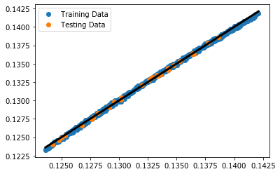
Parity Plot

plt.plot(y_train, y_train_predict, 'o', label='Training Data')
plt.plot(y_test, y_predict, 'o', label='Testing Data')
plt.plot([np.min(y_train), np.max(y_train)], [np.min(y_train), np.max(y_train)], color='k', lw=3)
plt.legend();

Predict Local Properties

This section predicts local properties using the LocalizationRegressor. The model can be trained using only a delta microstructure.

Generate the Data

Delta Data

Generate the delta data to fit the model.

x_delta = generate_delta(n_phases=2, shape=(21, 21)).persist()

#PYTEST_VALIDATE_IGNORE_OUTPUT

x_delta

Array Chunk Bytes 7.06 kB 7.06 kB Shape (2, 21, 21) (2, 21, 21) Count 1 Tasks 1 Chunks Type int64 numpy.ndarray

The y_delta data is also required to fit the model and is generated using a FE simulation.

y_delta = solve_fe(x_delta,
                   elastic_modulus=(100, 150),
                   poissons_ratio=(0.3, 0.3),
                   macro_strain=0.001)['strain'][..., 0].persist()

#PYTEST_VALIDATE_IGNORE_OUTPUT

y_delta

Array Chunk Bytes 7.06 kB 7.06 kB Shape (2, 21, 21) (2, 21, 21) Count 1 Tasks 1 Chunks Type float64 numpy.ndarray

Test Data

Generate the test data to test the model.

da.random.seed(2341234)

x_test = da.random.randint(2, size=(1,) + x_delta.shape[1:]).persist()
y_test = solve_fe(x_test,
                  elastic_modulus=(100, 150),
                  poissons_ratio=(0.3, 0.3),
                  macro_strain=0.001)['strain'][..., 0].persist()

Fit the Model

Generate the pipeline and fit the delta microstructure and predicted strain field.

model = Pipeline(steps=[
    ('discretize', PrimitiveTransformer(n_state=2, min_=0.0, max_=1.0)),
    ('regressor', LocalizationRegressor())
])

model.fit(x_delta, y_delta);

The model is calibrated so can now be used to predict the test data

y_predict = model.predict(x_test)

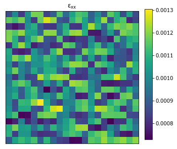
Plot the test data.

plot_microstructures(x_test[0], cmap='gray', colorbar=False);

plot_microstructures(y_test[0], titles='$\epsilon_{xx}$');

Compare the predicted and test results

plot_microstructures(y_test[0], y_predict[0], titles=['FE', 'MKS']);

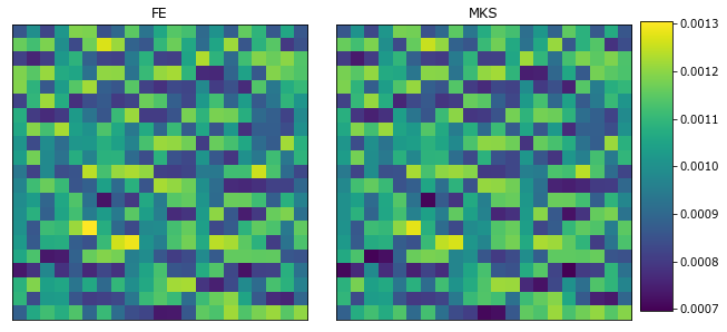
The LocalizationRegressor works well when the mapping is mostly linear (e.g. linear elasticity) where the contrast in materials properties is not too large.