Linear Elasticity in 2D

Introduction

This example provides a demonstration of using PyMKS to compute the linear strain field for a two-phase composite material. The example introduces the governing equations of linear elasticity, along with the boundary conditions required for the MKS. It subsequently demonstrates how to generate data for delta microstructures and then use this data to calibrate the first order MKS influence coefficients for all strain fields. The calibrated influence coefficients are used to predict the strain response for a random microstructure and the results are compared with those from finite element. Finally, the influence coefficients are scaled up and the MKS results are again compared with the finite element data for a large problem.

PyMKS uses the finite element tool SfePy to generate both the strain fields to fit the MKS model and the verification data to evaluate the MKS model’s accuracy.

Elastostatics Equations

For the sake of completeness, a description of the equations of linear elasticity is included. The constitutive equation that describes the linear elastic phenomena is Hook’s law.

\[\sigma_{ij} = C_{ijkl}\varepsilon_{kl}\]

\(\sigma\) is the stress, \(\varepsilon\) is the strain, and \(C\) is the stiffness tensor that relates the stress to the strain fields. For an isotropic material the stiffness tensor can be represented by lower dimension terms which can relate the stress and the strain as follows.

\[\sigma_{ij} = \lambda \delta_{ij} \varepsilon_{kk} + 2\mu \varepsilon_{ij}\]

\(\lambda\) and \(\mu\) are the first and second Lame parameters and can be defined in terms of the Young’s modulus \(E\) and Poisson’s ratio \(\nu\) in 2D.

\[\lambda = \frac{E\nu}{(1-\nu)(1-2\nu)}\]

\[\mu = \frac{E}{3(1+\nu)}\]

Linear strain is related to displacement using the following equation.

\[\varepsilon_{ij} = \frac{u_{i,j}+u_{j,i}}{2}\]

We can get an equation that relates displacement and stress by plugging the equation above back into our expression for stress.

\[\sigma_{ij} = \lambda u_{k,k} + \mu( u_{i,j}+u_{j,i})\]

The equilibrium equation for elastostatics is defined as

\[\sigma_{ij,j} = 0\]

and can be cast in terms of displacement.

\[\mu u_{i,jj}+(\mu + \lambda)u_{j,ij}=0\]

In this example, a displacement controlled simulation is used to calculate the strain. The domain is a square box of side \(L\) which has an macroscopic strain \(\bar{\varepsilon}_{xx}\) imposed.

In general, generating the calibration data for the MKS requires boundary conditions that are both periodic and displaced, which are quite unusual boundary conditions and are given by:

\[u(L, y) = u(0, y) + L\bar{\varepsilon}_{xx}\]

\[u(0, L) = u(0, 0) = 0\]

\[u(x, 0) = u(x, L)\]

Modeling with MKS

Calibration Data and Delta Microstructures

The first order MKS influence coefficients are all that is needed to compute a strain field of a random microstructure, as long as the ratio between the elastic moduli (also known as the contrast) is less than 1.5. If this condition is met, we can expect a mean absolute error of 2% or less, when comparing the MKS results with those computed using finite element methods [1].

Because we are using distinct phases and the contrast is low enough to only need the first order coefficients, delta microstructures and their strain fields are all that we need to calibrate the first order influence coefficients [2].

from sklearn.pipeline import Pipeline
import dask.array as da
import numpy as np

from pymks import (
    generate_delta,
    plot_microstructures,
    solve_fe,
    PrimitiveTransformer,
    LocalizationRegressor,
    coeff_to_real
)

#PYTEST_VALIDATE_IGNORE_OUTPUT

%matplotlib inline
%load_ext autoreload
%autoreload 2

The autoreload extension is already loaded. To reload it, use:
  %reload_ext autoreload

Here we use the generate_delta function to create the two delta microstructures needed to calibrate the first order influence coefficients.

x_delta = generate_delta(n_phases=2, shape=(21, 21)).persist()
plot_microstructures(x_delta[0], x_delta[1], titles=("X[0]", "X[1]"), cmap='gray');

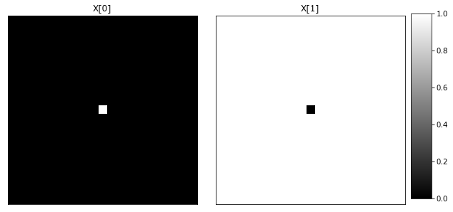
Using delta microstructures for the calibration of the first order influence coefficients is essentially the same as using a unit impulse response to find the kernel of a system in signal processing. Any given delta microstructure is composed of only two phases with the center cell having an alternative phase from the remainder of the domain.

Generating Calibration Data

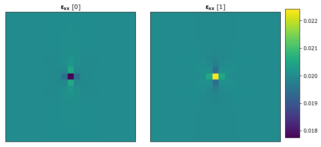
The solve_fe function provides an interface to generate strain fields, which can then be used for calibration of the influence coefficients.

This example uses a microstructure with elastic moduli values of 100 and 120 and Poisson’s ratio values of 0.3 and 0.3, respectively. The macroscopic imposed strain equal to 0.02. These parameters must be passed into the solve_fe function.

strain_xx = lambda x: solve_fe(
        x,
        elastic_modulus=(100, 120),
        poissons_ratio=(0.3, 0.3),
        macro_strain=0.02
    )['strain'][...,0]

y_delta = strain_xx(x_delta).persist()

Observe the strain fields.

plot_microstructures(
    y_delta[0],
    y_delta[1],
    titles=(r'$\mathbf{\varepsilon_{xx}}$ [0]', r'$\mathbf{\varepsilon_{xx}}$ [1]')
);

Calibrating First Order Influence Coefficients

The following creates a model using an Scikit-learn pipeline using the PrimitiveTransformer to discretize and the LocalizationRegressor to perform regression in Fourier space. n_state is set to 2 as there are 2 states.

model = Pipeline(steps=[
    ('discretize', PrimitiveTransformer(n_state=2, min_=0.0, max_=1.0)),
    ('regressor', LocalizationRegressor())
])

The delta microstructures are used to calibrate the influence coefficients.

model.fit(x_delta, y_delta);

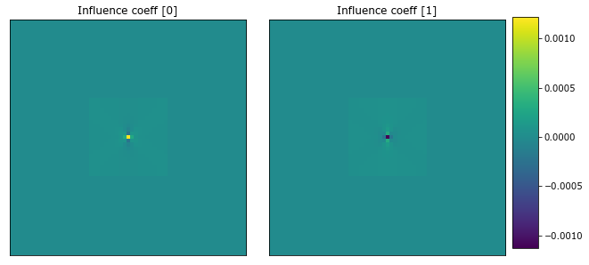
The influence coefficient have been calibrated. The influence coefficients need to be converted into real space to view. A helper function, to_real, is used to get the real space coefficients from the model.

to_real = lambda x: coeff_to_real(x.steps[1][1].coeff).real

coeff = to_real(model)
plot_microstructures(coeff[...,0], coeff[...,1], titles=['Influence coeff [0]', 'Influence coeff [1]']);

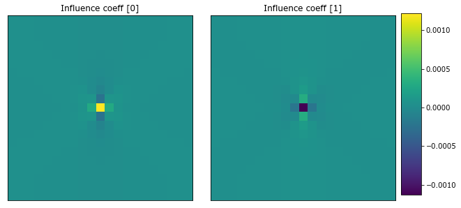
The influence coefficients have a Gaussian-like shape.

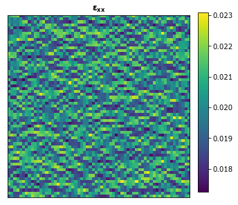
Predict the Strain Field for a Random Microstructure

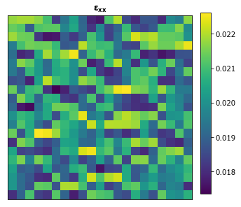
Let’s use the calibrated model to compute the strain field for a random two phase microstructure and compare it with the results from a finite element simulation. The strain_xx helper function is used to generate the strain field.

da.random.seed(99)

x_data = da.random.randint(2, size=(1,) + x_delta.shape[1:]).persist()
y_data = strain_xx(x_data).persist()

plot_microstructures(y_data[0], titles=[r'$\mathbf{\varepsilon_{xx}}$']);

Note that the calibrated influence coefficients can only be used to reproduce the simulation with the same boundary conditions that they were calibrated with.

Get the predicted strain field using model.predict.

y_predict = model.predict(x_data)

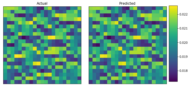
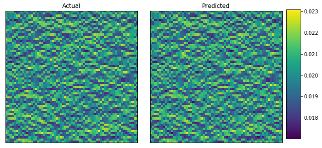
Finally, compare the results from finite element simulation and the MKS model.

plot_microstructures(y_data[0], y_predict[0], titles=['Actual', 'Predicted']);

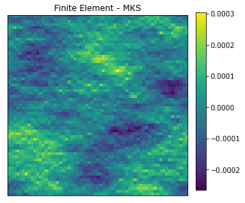
Lastly, observe the difference between the two strain fields.

plot_microstructures(y_data[0] - y_predict[0], titles=['Finite Element - MKS']);

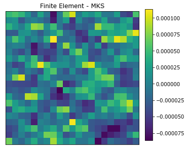
The MKS model is able to capture the strain field for the random microstructure after being calibrated with delta microstructures.

Resizing the Coefficients to use on Larger Microstructures

The influence coefficients that were calibrated on a smaller microstructure can be used to predict the strain field on a larger microstructure though spectral interpolation [3], but accuracy of the MKS model drops slightly. To demonstrate how this is done, generate a new random microstructure that is 3x larger

new_shape = tuple(np.array(x_delta.shape[1:]) * 3)
x_large = da.random.randint(2, size=(1,) + new_shape).persist()
y_large = strain_xx(x_large).persist()

plot_microstructures(y_large[0], titles=[r'$\mathbf{\varepsilon_{xx}}$']);

The influence coefficients that have already been calibrated need to be resized to match the shape of the new larger microstructure that we want to compute the strain field for. This can be done by passing the shape of the new larger microstructure into the resize_coeff method.

model.steps[1][1].coeff_resize(x_large[0].shape);

Observe the resized influence coefficients.

coeff = to_real(model)
plot_microstructures(coeff[...,0], coeff[...,1], titles=['Influence coeff [0]', 'Influence coeff [1]']);

The coefficients have been resized so will only work on the 63x63 microstructures. As before, pass the microstructure as the argument to the predict method to get the strain field.

y_predict_large = model.predict(x_large).persist()

plot_microstructures(y_large[0], y_predict_large[0], titles=['Actual', 'Predicted']);

Observe the difference between the two strain fields.

plot_microstructures(y_large[0] - y_predict_large[0], titles=['Finite Element - MKS']);

The results from the strain field computed with the resized influence coefficients are not as accurate, but still acceptable for engineering purposes. This decrease in accuracy is expected when using spectral interpolation [4].

References

[1] Binci M., Fullwood D., Kalidindi S.R., A new spectral framework for establishing localization relationships for elastic behavior of composites and their calibration to finite-element models. Acta Materialia, 2008. 56 (10) p. 2272-2282 doi:10.1016/j.actamat.2008.01.017.

[2] Landi, G., S.R. Niezgoda, S.R. Kalidindi, Multi-scale modeling of elastic response of three-dimensional voxel-based microstructure datasets using novel DFT-based knowledge systems. Acta Materialia, 2009. 58 (7): p. 2716-2725 doi:10.1016/j.actamat.2010.01.007.

[3] Marko, K., Kalidindi S.R., Fullwood D., Computationally efficient database and spectral interpolation for fully plastic Taylor-type crystal plasticity calculations of face-centered cubic polycrystals. International Journal of Plasticity 24 (2008) 1264–1276 doi:10.1016/j.ijplas.2007.12.002.

[4] Marko, K. Al-Harbi H. F. , Kalidindi S.R., Crystal plasticity simulations using discrete Fourier transforms. Acta Materialia 57 (2009) 1777–1784 doi:10.1016/j.actamat.2008.12.017.