Filter Example

This example demonstrates the connection between MKS and signal processing for a 1D filter. It shows that the filter is in fact the same as the influence coefficients and, thus, applying the LocalizationRegressor is in essence just applying a filter.

%load_ext autoreload
%autoreload 2

import numpy as np
import matplotlib.pyplot as plt
import scipy.ndimage
from sklearn.pipeline import Pipeline

from pymks import (
    PrimitiveTransformer,
    LocalizationRegressor,
    coeff_to_real
)

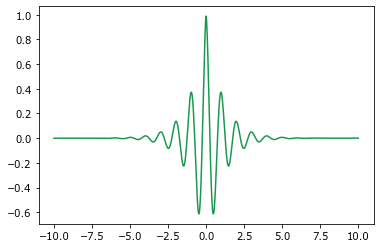
Construct a filter, \(F\), such that

\[F\left(x\right) = e^{-|x|} \cos{\left(2\pi x\right)}\]

Try to show that, if \(F\) is used to generate sample calibration data for the MKS, then the calculated influence coefficients are in fact just \(F\).

def filter_(x):
    return np.exp(-abs(x)) * np.cos(2 * np.pi * x)

x = np.linspace(-10.0, 10.0, 1000)
y = filter_(x)

plt.plot(x, y, color='#1a9850');

Next, generate the sample data using scipy.ndimage.convolve. This performs the convolution

\[p\left[ s \right] = \sum_r F\left[r\right] X\left[r - s\right]\]

for each sample.

np.random.seed(201)

def convolve(x_sample):
    return scipy.ndimage.convolve(
        x_sample,
        filter_(np.linspace(-10.0, 10.0, len(x_sample))),
        mode="wrap"
    )

x_data = np.random.random((50, 101))

y_data = np.array([convolve(x_sample) for x_sample in x_data])

print(x_data.shape, y_data.shape)

(50, 101) (50, 101)

For this problem, a basis is unnecessary, as no discretization is required in order to reproduce the convolution with the MKS localization. Using the PrimitiveTransformer with n_state=2 is the equivalent of a non-discretized convolution in space.

pipeline = Pipeline(steps=[
    ('discretize', PrimitiveTransformer(n_state=2)),
    ('regressor', LocalizationRegressor())
])

pipeline.fit(x_data, y_data)
y_predict = pipeline.predict(x_data)
fcoeff = pipeline.steps[1][1].coeff

print(y_predict[0, :4].compute())
print(y_data[0, :4])
print(fcoeff.shape)

[-0.41059557  0.20004566  0.61200171  0.5878077 ]
[-0.41059557  0.20004566  0.61200171  0.5878077 ]
(101, 2)

x = np.linspace(-10.0, 10.0, 101)
coeff = coeff_to_real(fcoeff, (101,))
plt.plot(x, filter_(x), label=r'$F$', color='#1a9850')
plt.plot(x, -coeff.real[:, 0] + coeff.real[:, 1],
         'k--', label=r'$\alpha$')
l = plt.legend()
plt.show()

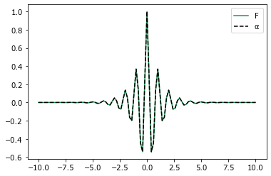
Some manipulation of the coefficients is required to reproduce the filter. Remember the convolution for the MKS is

\[p \left[s\right] = \sum_{l=0}^{L-1} \sum_{r=0}^{S - 1} \alpha[l, r] m[l, s - r]\]

However, when the primitive basis is selected, the MKSLocalizationModel solves a modified form of this. There are always redundant coefficients since

\[\sum\limits_{l=0}^{L-1} m[l, s] = 1\]

Thus, the regression in Fourier space must be done with categorical variables, and the regression takes the following form:

\[\begin{split} \begin{split} p [s] & = \sum_{l=0}^{L - 1} \sum_{r=0}^{S - 1} \alpha[l, r] m[l, s -r] \\ P [k] & = \sum_{l=0}^{L - 1} \beta[l, k] M[l, k] \\ &= \beta[0, k] M[0, k] + \beta[1, k] M[1, k] \end{split}\end{split}\]

where

\[\begin{split}\beta[0, k] = \begin{cases} \langle F(x) \rangle ,& \text{if } k = 0\\ 0, & \text{otherwise} \end{cases}\end{split}\]

This removes the redundancies from the regression, and we can reproduce the filter.