Using GraSPI
Reproduce Previous Work
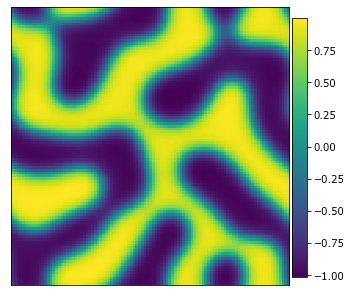
This notebook reproduces an analysis from the original GraSPI package. The microstructure is generated by a Cahn-Hilliard simulation. The graph statistics are designed to characterize a photo-voltaic device. The upper boundary is an anode and the bottom boundary is a cathode. The yellow material is donor while the blue material is acceptor.
[7]:
import pandas
import numpy as np
import dask.array as da
from dask.distributed import Client
from dask_ml.preprocessing import MinMaxScaler
from dask_ml.linear_model import LogisticRegression
from dask_ml.model_selection import train_test_split
from sklearn.pipeline import Pipeline
from sklearn.feature_selection import VarianceThreshold
from sklearn.metrics import confusion_matrix
from toolz.curried import pipe, curry

from pymks import (
    solve_cahn_hilliard,
    plot_microstructures,
    graph_descriptors,
    GenericTransformer,
    GraphDescriptors
)
[8]:
data = np.array(pandas.read_csv('data_0.528_3.8_000160.txt', delimiter=' ', header=None)).swapaxes(0, 1)
[9]:
plot_microstructures(data.swapaxes(0, 1), colorbar=False);

[10]:
data.shape
[10]:
(401, 101)
graph_descriptors works with Numpy arrays. The extra dimension is required as PyMKS functions require a sample axis. When using Numpy arrays graph_descriptors will return an ordinary Pandas dataframe (not Dask).
[11]:
graph_descriptors(data.reshape((1,) + data.shape))
[11]:
| n_vertices | n_edges | n_phase0 | n_phase1 | n_phase0_connect | n_phase1_connect | n_phase0_connect_top | n_phase1_connect_bottom | w_frac_phase0 | frac_phase0 | ... | inter_frac_bottom_and_top | frac_phase0_top | frac_phase1_bottom | n_inter_paths | n_phase0_inter_top | n_phase1_inter_bottom | frac_phase0_rising | frac_phase1_rising | n_phase0_connect_anode | n_phase1_connect_cathode | |
|---|---|---|---|---|---|---|---|---|---|---|---|---|---|---|---|---|---|---|---|---|---|
| 0 | 40501 | 3698 | 19268 | 21233 | 22 | 5 | 9 | 3 | 0.298392 | 0.475741 | ... | 0.296376 | 0.319545 | 0.979843 | 1096 | 1159 | 3668 | 0.522495 | 0.152944 | 207 | 196 |
1 rows × 22 columns
Generate Microstructures to Test Speed
Generate 144 microstructures to test speed with and without Dask
[12]:
#PYTEST_VALIDATE_IGNORE_OUTPUT

Client()
[12]:
Client
|
Cluster
|
Create 144 sample chunked into 6.
[18]:
da.random.seed(99)

n_sample = 144
n_domain = 101
n_chunks = 24

x_data = (
    2 * da.random.random((n_sample, n_domain, n_domain), chunks=(n_chunks, n_domain, n_domain)) - 1
)
y_data = solve_cahn_hilliard(x_data, delta_t=1.0, n_steps=100, delta_x=0.5).persist()
[19]:
plot_microstructures(y_data[0]);
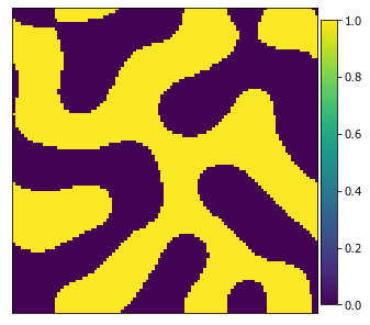
The graph descriptors function requies data binned into either 0 or 1 phases
[20]:
y_data_binned = da.where(y_data > 0, 1, 0).persist()
y_data_np = y_data_binned.compute()
[21]:
plot_microstructures(y_data_binned[0]);
On a laptop the Dask version is almost 5 times faster. Note that the graph_descriptors function returns a Numpy or Dask array based on whether its passed a Numpy array or Dask array. Passing it a Numpy array will force it to work as one process and therefore will be slower.
[22]:
#NBVAL_SKIP

%time out_pandas = graph_descriptors(y_data_np)
CPU times: user 519 ms, sys: 65.7 ms, total: 585 ms
Wall time: 19 s
[23]:
#NBVAL_SKIP

%time graph_descriptors(y_data_binned).compute()
CPU times: user 212 ms, sys: 6.21 ms, total: 219 ms
Wall time: 5.16 s
[23]:
| n_vertices | n_edges | n_phase0 | n_phase1 | n_phase0_connect | n_phase1_connect | n_phase0_connect_top | n_phase1_connect_bottom | w_frac_phase0 | frac_phase0 | ... | inter_frac_bottom_and_top | frac_phase0_top | frac_phase1_bottom | n_inter_paths | n_phase0_inter_top | n_phase1_inter_bottom | frac_phase0_rising | frac_phase1_rising | n_phase0_connect_anode | n_phase1_connect_cathode | |
|---|---|---|---|---|---|---|---|---|---|---|---|---|---|---|---|---|---|---|---|---|---|
| 0 | 10201 | 927 | 5039 | 5162 | 4 | 2 | 2 | 2 | 0.311396 | 0.493971 | ... | 0.437972 | 0.433022 | 1.000000 | 406 | 402 | 931 | 0.454629 | 0.148198 | 69 | 37 |
| 1 | 10201 | 951 | 5149 | 5052 | 3 | 4 | 1 | 1 | 0.326425 | 0.504754 | ... | 0.179811 | 0.774325 | 0.480008 | 171 | 688 | 446 | 0.403812 | 0.246186 | 73 | 31 |
| 2 | 10201 | 907 | 5135 | 5066 | 3 | 3 | 2 | 2 | 0.305060 | 0.503382 | ... | 0.127894 | 0.109056 | 0.897158 | 116 | 111 | 791 | 0.996429 | 0.049065 | 59 | 41 |
| 3 | 10201 | 942 | 5019 | 5182 | 4 | 1 | 2 | 1 | 0.307790 | 0.492011 | ... | 0.695329 | 0.698346 | 1.000000 | 655 | 653 | 950 | 0.276177 | 0.131030 | 51 | 52 |
| 4 | 10201 | 917 | 5142 | 5059 | 3 | 4 | 2 | 3 | 0.317781 | 0.504068 | ... | 0.731734 | 0.957021 | 0.783159 | 671 | 853 | 740 | 0.246698 | 0.220343 | 51 | 55 |
| ... | ... | ... | ... | ... | ... | ... | ... | ... | ... | ... | ... | ... | ... | ... | ... | ... | ... | ... | ... | ... | ... |
| 19 | 10201 | 959 | 5006 | 5195 | 5 | 2 | 1 | 1 | 0.313552 | 0.490736 | ... | 0.259645 | 0.329604 | 0.959769 | 249 | 301 | 921 | 0.329091 | 0.181508 | 48 | 58 |
| 20 | 10201 | 991 | 5065 | 5136 | 4 | 1 | 2 | 1 | 0.309485 | 0.496520 | ... | 0.501514 | 0.505429 | 1.000000 | 497 | 493 | 999 | 0.216016 | 0.125389 | 44 | 56 |
| 21 | 10201 | 944 | 5161 | 5040 | 2 | 4 | 1 | 2 | 0.317732 | 0.505931 | ... | 0.739407 | 0.920364 | 0.868849 | 698 | 854 | 798 | 0.215579 | 0.356246 | 25 | 78 |
| 22 | 10201 | 941 | 5178 | 5023 | 3 | 4 | 2 | 2 | 0.323143 | 0.507597 | ... | 0.676939 | 0.794515 | 0.942266 | 637 | 735 | 848 | 0.318182 | 0.227763 | 48 | 58 |
| 23 | 10201 | 961 | 5075 | 5126 | 3 | 2 | 2 | 2 | 0.305052 | 0.497500 | ... | 0.665973 | 0.637241 | 1.000000 | 640 | 636 | 965 | 0.174397 | 0.062037 | 53 | 45 |
144 rows × 22 columns
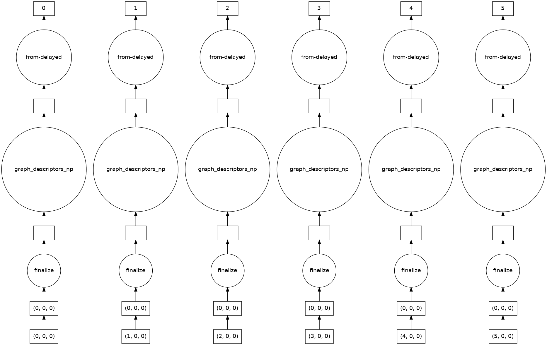
[24]:
#PYTEST_VALIDATE_IGNORE_OUTPUT

out = graph_descriptors(y_data_binned)
out.visualize()
[24]:
[25]:
#NBVAL_SKIP

from dask.distributed import performance_report

with performance_report(filename="dask-report.html"):
    out_pandas = out.compute()
[26]:
#NBVAL_SKIP

import IPython
IPython.display.HTML(filename='dask-report.html')
[26]:
Using Pipelines
Demonstrate how to use the graph descriptors as part of a machine learning pipeline. The GraphDescriptors object is a wrapper for the graph_descriptors function so that it works as part of a Scikit-learn pipeline.
Note that at this point it is a good idea to restart the notebook and only run the import cell and the Client cell above due to some memory issues.
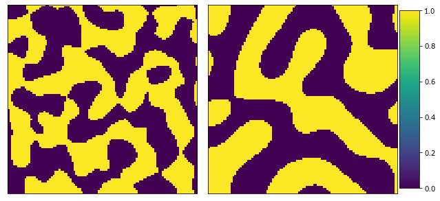
The following generates 96 x 2 samples each with a different Cahn-Hilliard microstructure. The microstructures differ based on the time of evolution (10 steps versus 100 steps). This is not a particularly great machine learning example, but suffices to demonstrate using GraphDescriptors as part of a pipeline.
[27]:
def generate_data(n_category, n_chunks, n_domain, seed=99):
    da.random.seed(seed)
    solve_ch = curry(solve_cahn_hilliard)(delta_t=1.0, delta_x=0.5)
    x_data = pipe(
        da.random.random((n_category * 2, n_domain, n_domain),
                         chunks=(n_chunks, n_domain, n_domain)),
        lambda x: 2 * x - 1,
        lambda x: [
            solve_ch(x[:n_category], n_steps=10),
            solve_ch(x[n_category:], n_steps=100)
        ],
        da.concatenate,
        lambda x: da.where(x > 0, 1, 0).persist()
    )
    y_data = da.from_array(
        np.concatenate([np.zeros(n_category), np.ones(n_category)]).astype(int),
        chunks=(n_chunks,)
    )
    return x_data, y_data
[28]:
n_category = 96
n_chunks = 24
n_domain = 101

x_data, y_data = generate_data(n_category, n_chunks, n_domain)
For demonstration purposes the data is “persisted” in memory meaning that Dask has calculated the memory and stored in chunks on each worker.
[29]:
#PYTEST_VALIDATE_IGNORE_OUTPUT

x_data
[29]:
|
[30]:
#PYTEST_VALIDATE_IGNORE_OUTPUT

y_data
[30]:
|
The second category is more evolved.
[31]:
plot_microstructures(x_data[0], x_data[n_category]);
The pipeline for fitting and predicting. The GenericTransformer allows to wrap simple transformer functions to reshape the data and remove unwanted features. The data needs to be flattened for use with train_test_split and then reshaped for use with GraphDescriptors. The MinMaxSclaler is used to rescale the graph descriptors feature to be between 0 and 1. Finally, LogisticRegression is used to classify the microstructures.
[32]:
pipeline = Pipeline(steps=[
    ('reshape', GenericTransformer(lambda x: x.reshape(x.shape[0], n_domain, n_domain))),
    ('descriptors', GraphDescriptors()),
    ('normalizer', MinMaxScaler()),
    ('to_array', GenericTransformer(lambda x: x.to_dask_array(lengths=True))),
    ('remove_features', GenericTransformer(lambda x: x[:, 1:])),
    ('decision', LogisticRegression())
])
train_test_split requires the x_data to be shaped as n_sample x n_features. A 20% test size is used.
[33]:
x_train, x_test, y_train, y_test = train_test_split(
    x_data.reshape(x_data.shape[0], -1),
    y_data,
    test_size=0.2
)
Fit the data. There have been some unresolved memory leaks at this stage. As noted above, reset the notebook before running this final section.
[34]:
# NBVAL_SKIP

pipeline.fit(x_train, y_train);
Make a prediction. y_predict is lazily evaluated so is an uncomputed Dask array at this stage. compute needs to be called to execute the prediction.
[35]:
# NBVAL_SKIP

y_predict = pipeline.predict(x_test)
Seems to be a perfect prediction.
[36]:
# NBVAL_SKIP

confusion_matrix(y_test.compute(), y_predict.compute())
[36]:
array([[20,  0],
       [ 0, 20]])
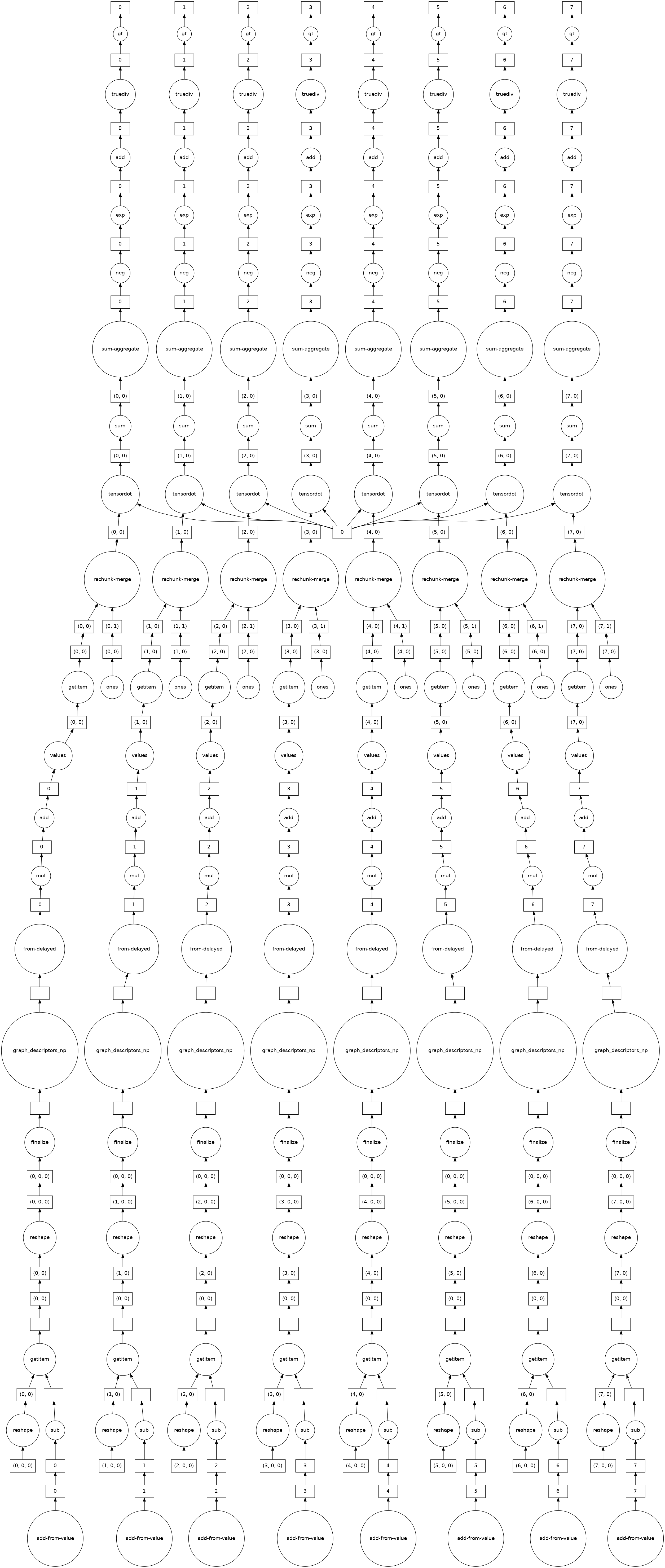
The entire prediction graph
[37]:
# NBVAL_SKIP

y_predict.visualize()
[37]:
[ ]: